Forecasting the tropical Pacific sea surface temperatures by nonlinear canonical correlation analysis

Aiming Wu and William W. Hsieh

The nonlinear canonical correlation analysis (NLCCA), developed by Hsieh (2000) using a neural network (NN) approach, has been applied to study the nonlinear relation between the tropical Pacific sea level pressure (SLP) and sea surface temperature (SST) fields (Hsieh, 2001), as well as between the wind stress and SST fields (Wu and Hsieh, 2001). Here the NLCCA model is used for the seasonal forecasts of the tropical Pacific SST from the SLP.

The monthly tropical Pacific SLP data (COADS, Woodruff et al. 1987) and the monthly tropical Pacific SST data (Smith et al. 1996) had their seasonal cycles and linear trends removed, and a 3-month running mean applied. Predictands are the 5 leading principal components (PCs) of the SST anomalies (SSTA). Predictors are the 7 leading PCs from the singular spectrum analysis (i.e. extended EOF) of the SLP anomalies with a 21-month lag window and a 3-month lag interval. The predictors and predictands are the inputs to the NLCCA model. Data from 1950 to 1989 were used for building (training) the model, and independent forecasts were made for the period from 1990 onward. The linear trend was added back to the predicted SSTA.

Due to local minima problems in finding nonlinear modes, only the leading NLCCA mode was used. From the residual data, the linear CCA was used to extract additional modes. At forecast lead times of 0 to 6 months, the nonlinear approach uses the leading NLCCA mode plus two more linear CCA modes, versus the linear approach with three CCA modes. For longer lead times (up to 15 months), the nonlinear approach uses 1 NLCCA mode plus 3 CCA modes, versus 4 CCA modes in the linear approach, as this achieves higher skills for both the nonlinear and linear approaches. Table 1 shows the forecasts skills from the nonlinear approach and from the linear approach.

Table 1. Correlation skills and root mean square errors (RMSE, in deg. C) over the Nino1+2, Nino3, Nino3.4 and Nino4 areas in the equatorial Pacific from forecasts by the nonlinear (NL) and the linear (CCA) approaches, for lead times from 0 to 15 months. Calculations were made for the period of 1990 to 2000.

                   Correlation                                RMSE
    ----------------------------------------------------------------------------
    lead  Nino1+2   Nino3  Nino3.4  Nino4        Nino1+2  Nino3  Nino3.4  Nino4
    ----------------------------------------------------------------------------
       0   0.763    0.881   0.923   0.898          0.72    0.40    0.31    0.27
       3   0.697    0.783   0.853   0.863          0.81    0.52    0.43    0.33
   NL  6   0.652    0.753   0.811   0.771          0.86    0.55    0.48    0.42
       9   0.552    0.655   0.715   0.746          0.93    0.66    0.60    0.43
      12   0.491    0.629   0.660   0.672          0.98    0.68    0.65    0.48
      15   0.380    0.524   0.535   0.522          1.07    0.77    0.76    0.58
    ----------------------------------------------------------------------------
       0   0.762    0.878   0.924   0.889          0.72    0.40    0.31    0.28
       3   0.648    0.757   0.844   0.862          0.85    0.55    0.44    0.31
   CCA 6   0.594    0.708   0.766   0.758          0.89    0.60    0.54    0.42
       9   0.507    0.631   0.719   0.758          0.96    0.67    0.59    0.42
      12   0.525    0.624   0.649   0.660          0.96    0.69    0.67    0.49
      15   0.409    0.513   0.515   0.498          1.07    0.79    0.79    0.61
    ----------------------------------------------------------------------------

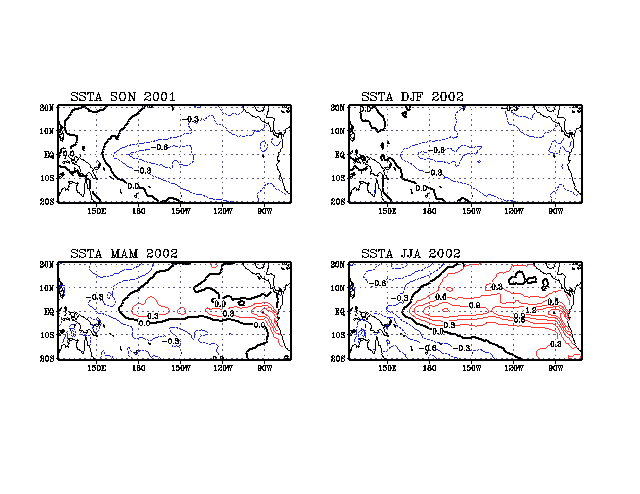
Using data up to the end of August, 2001, forecasts were made with the nonlinear approach. Forecasts for the SSTA in the Nino3.4 region at various lead times are shown in Fig.1, while the forecasted SSTA fields over the tropical Pacific are shown in Fig.2. For the fall and winter, slightly cool conditions are forecasted over the tropical Pacific. By spring and summer, 2002, warm conditions are forecasted to develop in the tropical Pacific.

Figure 1. The SST anomalies (SSTA) (in degree Celsius) in the Nino3.4 area (170W-120W, 5S-5N) predicted by the nonlinear model at 3, 6, 9 and 12 months of lead time (red solid line), with observations denoted by the dashed line. Tick marks along the abscissa indicate the January of the given years. (The postscript file of Fig.1 is also available).

Figure 2. SSTA (in degree Celsius) predicted by the nonlinear model at 3, 6, 9 and 12 months of lead time, corresponding to the fall (SON) of 2001, the winter (DJF), spring (MAM) and summer (JJA) of 2002, respectively. Positive SSTA are drawn with red solid contours and negative SSTA with blue dashed contours. Contour intervals are 0.3 C. (The postscript file of Fig.2 is also available).

In the near future, we will develop an ensemble forecast approach using the NLCCA, and cross-validate the forecast skills from 1950 to 2001.

References

Hsieh, W.W., 2000. Nonlinear canonical correlation analysis by neural networks. Neural Networks 13: 1095-1105.

Hsieh, W.W., 2001. Nonlinear canonical correlation analysis of the tropical Pacific climate variability using a neural network approach. J. Clim. 14: 2528-2539. (reprint in PDF or preprint in postscript).

Smith, T.M., Reynolds, R.W., Livezey, R.E. and Stokes, D.C., 1996. Reconstruction of historical sea surface temperatures using empirical orthogonal functions. J. Clim. 9: 1403-1420.

Woodruff, S.D., Slutz, R.J., Jenne, R.L. and Steurer, P.M., 1987. A comprehensive ocean-atmosphere data set. Bull. Amer. Meteorol. Soc. 6: 1239-1250.

Wu, A. and Hsieh, W.W., 2001. Nonlinear canonical correlation analysis of the tropical Pacific wind stress and sea surface temperature (Submitted to Clim. Dynam.).